Exploratory Data Analysis
Exploratory Data Analysis or EDA is one of the most important steps in the model building process. During EDA you learn about the data that you have available to you. A few of the more common EDA questions are included below:
-
Does the data have missing values?
-
Does the data contain outliers?
-
How is the data distributed?
-
Does the data have any odd trends over time?
-
Are the variables related to each other? (Correlation or covariance)
-
Are there other features we could create that would benefit the model?
We’ll attempt to answer some of these questions in this section. However, EDA is always evolving and isn’t a one size fits all process. It’s important to think critically about your data and what you want to know. Don’t just follow the questions above any think that you are done with EDA.
|
This section is written with Python in mind. However, R and other languages should have duplicate functionalities for most, if not all, of the items mentioned below. |
Data Understanding
In most EDA processes the very first step is getting familiar with the data set. What are the column names, how is it indexed, what is the unit of measurement (UoM) for each variable? All of these are valid questions that the analyst will need to understand.
Once a very basic understanding is formed it’s time to jump into the data. This often consists of:
-
Checking for missing values.
-
Checking of outliers.
-
Time series visualizations (if applicable).
-
Category visualizations (if applicable).
These examples use The Data Mine’s olympics data set, but the concepts should apply to almost any data.
In this hypothetical case let’s say that our goal is to predict if the athlete is going to win a gold medal. That would make it a classification problem. We want to predict 1 if gold and 0 for everything else.
We can start by printing out the data:
import pandas as pd
init_data = pd.read_csv('/depot/datamine/data/olympics/athlete_events.csv')
print(init_data.head())
ID Name Sex Age Height Weight Team \
0 1 A Dijiang M 24.0 180.0 80.0 China
1 2 A Lamusi M 23.0 170.0 60.0 China
2 3 Gunnar Nielsen Aaby M 24.0 NaN NaN Denmark
3 4 Edgar Lindenau Aabye M 34.0 NaN NaN Denmark/Sweden
4 5 Christine Jacoba Aaftink F 21.0 185.0 82.0 Netherlands
NOC Games Year Season City Sport \
0 CHN 1992 Summer 1992 Summer Barcelona Basketball
1 CHN 2012 Summer 2012 Summer London Judo
2 DEN 1920 Summer 1920 Summer Antwerpen Football
3 DEN 1900 Summer 1900 Summer Paris Tug-Of-War
4 NED 1988 Winter 1988 Winter Calgary Speed Skating
Event Medal
0 Basketball Men's Basketball NaN
1 Judo Men's Extra-Lightweight NaN
2 Football Men's Football NaN
3 Tug-Of-War Men's Tug-Of-War Gold
4 Speed Skating Women's 500 metres NaN
For any of the numeric columns we can easily find missing values by using the pandas describe() function. This is also one of the first times we can check for outliers.
print(init_data.describe()) ID Age Height Weight \
count 271116.000000 261642.000000 210945.000000 208241.000000
mean 68248.954396 25.556898 175.338970 70.702393
std 39022.286345 6.393561 10.518462 14.348020
min 1.000000 10.000000 127.000000 25.000000
25% 34643.000000 21.000000 168.000000 60.000000
50% 68205.000000 24.000000 175.000000 70.000000
75% 102097.250000 28.000000 183.000000 79.000000
max 135571.000000 97.000000 226.000000 214.000000
Year
count 271116.000000
mean 1978.378480
std 29.877632
min 1896.000000
25% 1960.000000
50% 1988.000000
75% 2002.000000
max 2016.000000
First thing we can see that Age, Height, and Weight are all missing values. Interestingly we can also see a potential outlier in the Age column with a max value of 97. These are all things that we’ll check into, but for now we can also check the text variables.
for c in init_data.columns:
    data_type = init_data[c].dtype
    if(data_type != 'int64') & (data_type != 'float64'):
        count_of_null = sum(init_data[c].isna())
        print("Column {} has {} null values.".format(c, count_of_null))
Column Name has 0 null values. Column Sex has 0 null values. Column Team has 0 null values. Column NOC has 0 null values. Column Games has 0 null values. Column Season has 0 null values. Column City has 0 null values. Column Sport has 0 null values. Column Event has 0 null values. Column Medal has 231333 null values.
We can double check this if we want by using the unique() function.
print(init_data['Games'].unique())['1992 Summer' '2012 Summer' '1920 Summer' '1900 Summer' '1988 Winter' '1992 Winter' '1994 Winter' '1932 Summer' '2002 Winter' '1952 Summer' '1980 Winter' '2000 Summer' '1996 Summer' '1912 Summer' '1924 Summer' '2014 Winter' '1948 Summer' '1998 Winter' '2006 Winter' '2008 Summer' '2016 Summer' '2004 Summer' '1960 Winter' '1964 Winter' '1984 Winter' '1984 Summer' '1968 Summer' '1972 Summer' '1988 Summer' '1936 Summer' '1952 Winter' '1956 Winter' '1956 Summer' '1960 Summer' '1928 Summer' '1976 Summer' '1980 Summer' '1964 Summer' '2010 Winter' '1968 Winter' '1906 Summer' '1972 Winter' '1976 Winter' '1924 Winter' '1904 Summer' '1928 Winter' '1908 Summer' '1948 Winter' '1932 Winter' '1936 Winter' '1896 Summer']
The lack of NaN or Null in the output above confirms that our code to check for missing values in the text variables worked as expected.
Now that we have an idea of the variables that are missing we can go back to see if we can better understand why they may be missing. In this example we’ll look at Age, but you should check any variable that may be of interest.
no_age = init_data.loc[init_data['Age'].isna() == True]
print(no_age.head(1))
ID Name Sex Age Height Weight Team NOC \
147 54 Mohamed Jamshid Abadi M NaN NaN NaN Iran IRI
Games Year Season City Sport Event Medal
147 1948 Summer 1948 Summer London Boxing Boxing Men's Heavyweight NaN
My first thought is that maybe it’s due to when the records were recorded. Maybe before a certain year they didn’t record Age. We should be able to check that pretty quickly.
print(no_age['Year'].min(), no_age['Year'].max())1896 2008
It looks like records don’t have an age from the 1800’s all the way through 2008 so it’s likely not due to how old they are.
For the purposes of this demonstration I’m not going to dig further into the Age column, but this illustrates one of the core components of EDA. Ask questions and make hypotheses of your data and then use the data to prove or disprove them. This helps you learn and think about how you may use the data.
Data Relationships
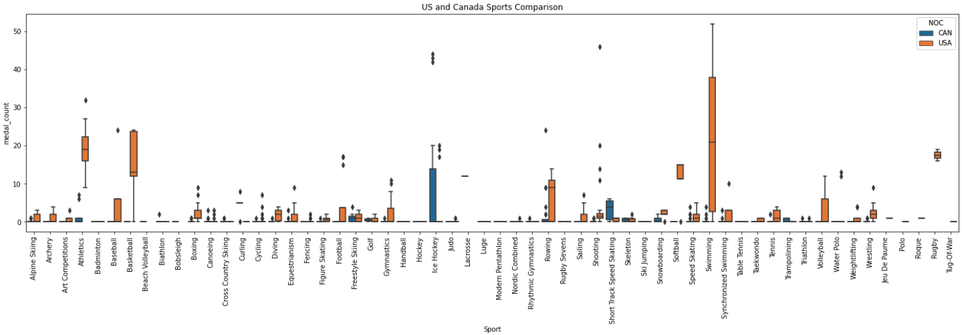
After you’ve built a basic understanding of each variable, you’ll often start to dig in to how they are related to each other or how they change over time. The example below shows an example of how you may be interested to see differences in gold medals by different variables.
For this example, I cut down the data to compare the medal counts by sport for the United States and Canada. This graph helps to illustrate lots of different information. The Sport variable seems to really be differentiated by Team. These may be valuable variables to include in the model.
import seaborn as sns
import matplotlib.pyplot as plt
import numpy as np

# Cutting down the data for the example.
us_and_canada = init_data.loc[init_data['Team'].str.lower().isin(['canada', 'united states'])].copy()
us_and_canada['medal_count'] = np.where(us_and_canada['Medal'].str.lower() == 'gold', 1, 0)
us_and_canada_grouped_year = us_and_canada.groupby(['NOC', 'Sport', 'Year']).agg({'medal_count': 'sum'}).reset_index()

fig, ax1 = plt.subplots(1,1, figsize=(25,6))

sns.boxplot(x='Sport', y='medal_count', hue='NOC', data=us_and_canada_grouped_year, ax=ax1)
plt.xticks(rotation=90)
plt.title("US and Canada Sports Comparison")

plt.show()
plt.close('all')
Data Over Time
In the same way that we look at groups of data it’s often helpful to look at data over time. This can show relationships that we may not have been aware of. These types of variables can also be included in a model.
For example, going back to the Olympic data that we are working with we could hypothesize that the number of medals in the last Olympics may be a good predictor of medals in this Olympics. If we wanted to check this quickly in a graph, we could plot the medals over time for a few different nations. If we see a ton of variation (very spiky plot) then maybe it isn’t a great predictor. However, if we see that countries tend to keep similar trends then maybe it’s worth including in the model.
# Let's choose a few countries to compare. In this case we'll limit to the summer games.
data_subset = init_data.loc[(init_data['NOC'].isin(['CHN','DEN','NED','USA','FIN']) & (init_data['Season'] == 'Summer'))].copy()

data_subset['medal_count'] = np.where(data_subset['Medal'].isna(), 0, 1)
grouped_data = data_subset.groupby(['NOC', 'Year']).agg({'medal_count': 'sum'}).reset_index()

# Just to make sure it graphs correctly we'll sort the data.
grouped_data = grouped_data.sort_values(by=['NOC', 'Year'])

# Now we can plot over time!
fig, ax1 = plt.subplots(1, 1, figsize=(20,8))

# Set plot information
ax1.set_title('Country Medals by Year')
ax1.set_xlabel('Year')
ax1.set_ylabel('Total Medals')

# China
chn_data = grouped_data.loc[grouped_data['NOC'] == 'CHN']
ax1.plot(chn_data['Year'], chn_data['medal_count'], c='red', label='China')

# Denmark
den_data = grouped_data.loc[grouped_data['NOC'] == 'DEN']
ax1.plot(den_data['Year'], den_data['medal_count'], c='blue', label='Denmark')

# Netherlands
ned_data = grouped_data.loc[grouped_data['NOC'] == 'NED']
ax1.plot(ned_data['Year'], ned_data['medal_count'], c='grey', label='Netherlands')

# USA
usa_data = grouped_data.loc[grouped_data['NOC'] == 'USA']
ax1.plot(usa_data['Year'], usa_data['medal_count'], c='purple', label='USA')

# Finland
fin_data = grouped_data.loc[grouped_data['NOC'] == 'FIN']
ax1.plot(fin_data['Year'], fin_data['medal_count'], c='green', label='Finland')

# Add the key for reference
plt.legend()

plt.show()
plt.close('all')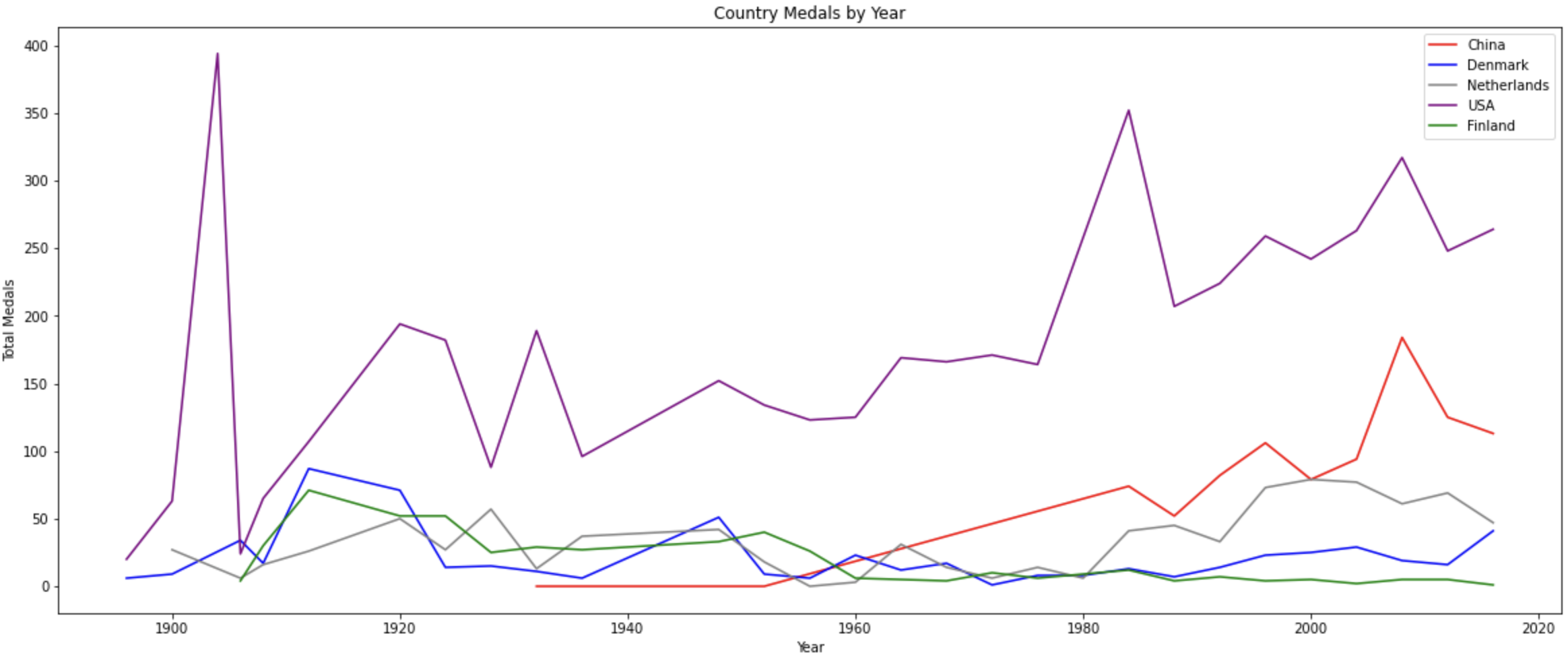
In this case we see that there is some variance over time with respect to the country. The United States has a large spike at the very beginning and then a steady upward trend. This shows that the last Olympics' medals alone may not be the best predictor. However, we could potentially create a variable that shows the historical trend for the country. That could be very helpful. These are all items that you can test with your modeling process!
Correlation and Covariance
Correlation and covariance are two very common terms in the world of analytics. At their core they both show how two variables relate to one another. A few great resources for understanding correlation and covariance are included below:
Rather than try to explain a topic that’s already well-covered online, our goal is to guide you through code to test the concept yourself.
We can start by generating a bit of random data. To do this we can actually use a covariance matrix.
The covariance matrix will show the relationship between the different variables. On the diagonal you’ll find the variance for each measurement. The off-diagonal elements show the covariance values. In this case the larger the value (positive or negative) the more the variables appear to move in the same pattern.
Variable 1 |
Variable 2 |
Variable 3 |
|
Variable 1 |
150 |
360 |
-50 |
Variable 2 |
360 |
100 |
0 |
Variable 3 |
-50 |
0 |
110 |
In this example the table shows us the variance of Variable 1 is 150, Variable 2 is 100, and Variable 3 is 110. If you’re not familiar with variance it’s always good to go back and review.
We can use the same matrix in the code below to generate a number of data points based on the variance and covariance in our matrix.
import pandas as pd
import seaborn as sns
import matplotlib.pyplot as plt
import numpy as np
covariance_matrix = [
[504, 360, -200],
[360, 360, 0],
[-200, 0, 720]
]
mean_to_use = [0, 0, 0]
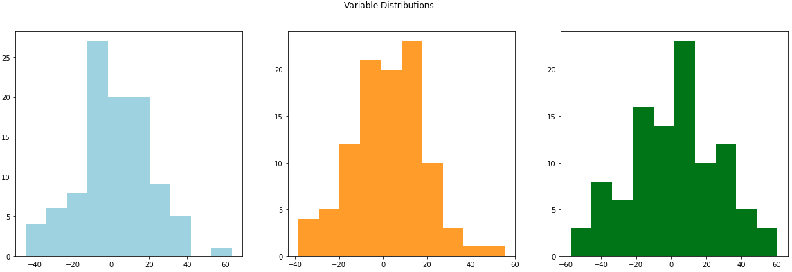
example_data = np.random.multivariate_normal(mean_to_use, covariance_matrix, size=100)
dataframe_example_data = pd.DataFrame(example_data, columns=["variable_1", "variable_2", "variable_3"])We can plot these new variables with histograms to see how they are distributed. In this case we’ll see that they match with the mean of 0 that we passed in with mean_to_use. You’ll also notice that if you go back and change the variance (diagonal elements in the matrix) the width of the distribution will change.
If we generate scatter plots we’d expect the visual trends to match our covariance matrix input. In this case Variable 1 and Variable 2 should have a strong positive trend (360). Variable 1 and Variable 3 should have a negative trend (-200). Variable 2 and Variable 3 should have little to no trend (0).
fig, (ax1, ax2, ax3) = plt.subplots(1, 3, figsize=(20,6))

ax1.scatter(dataframe_example_data['variable_1'], dataframe_example_data['variable_2'], color='lightblue')
ax2.scatter(dataframe_example_data['variable_1'], dataframe_example_data['variable_3'], color='orange')
ax3.scatter(dataframe_example_data['variable_2'], dataframe_example_data['variable_3'], color='green')

ax1.set_title("Variable 1 and Variable 2")
ax2.set_title("Variable 1 and Variable 3")
ax3.set_title("Variable 2 and Variable 3")

plt.show()
plt.close('all')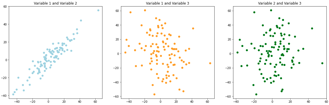
We see the positive, negative, and no trend graphs that we’d expect! Although as the articles mention this can be a bit hard to interpret. For example, how does 360 compare to -200. Correlation helps to fix this by standardizing the data. This puts all of the values on the same scale between -1 and 1. Pandas has an easy built-in function to check the correlation of our values.
print(dataframe_example_data.corr())variable_1 variable_2 variable_3 variable_1 1.000000 0.928896 -0.271224 variable_2 0.928896 1.000000 0.090006 variable_3 -0.271224 0.090006 1.000000
We can see that this follows the same positive, negative, and no-trend patterns as a covariance matrix, but it’s a little easier to understand on this scale.
Now it’s your turn! Play with the code above to see how the different values change as you input different variables.
Imputation
Imputation is a very common topic when working with data. Often, the data is missing a large number of samples and we have to decide what to do with them.
If there are a small number of samples missing you may just remove those rows. Although, it should be noted that it is important to understand why the samples are missing in the first place.
If there is a large number of samples missing or you are trying to add data to the data set, you may end up imputing values.
Just like with correlation and covariance there is a ton of great content already written around these topics online. Usually you’ll find a few simple techniques, such as mean imputation, and a few more complicated techniques, such as SMOTE.
We encourage you to do your own digging to learn more about imputation. In this section we’ll focus on helping to highlight some of the risks of imputation as well as how we can use interactive learning to understand the different imputation techniques.
To illustrate one of the risks of imputation we can go back to our Olympics dataset and check the Weight variable.
import pandas as pd
import seaborn as sns
import matplotlib.pyplot as plt
import numpy as np

init_data = pd.read_csv('/depot/datamine/data/olympics/athlete_events.csv')

fig, ax1 = plt.subplots(1, 1, figsize=(8,6))

ax1.hist(init_data['Weight'], bins=50)
ax1.set_title("Weight Variable")

plt.show()
plt.close('all')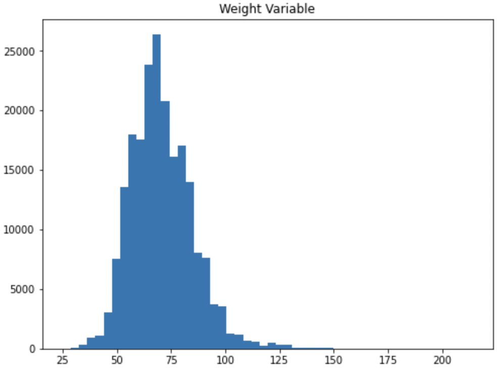
We know from the EDA that we did above that the variable has missing values. Many times with imputation it’s tempting to say we can just add the average. After all, it’s the average for everyone at the Olympics so it shouldn’t be too bad to use that value right?
init_data['imputed_weight'] = np.where(init_data['Weight'].isna(), init_data['Weight'].mean(), init_data['Weight'])

fig, ax1 = plt.subplots(1, 1, figsize=(8,6))

ax1.hist(init_data['imputed_weight'], bins=50)
ax1.set_title('Imputed Weight')

plt.show()
plt.close('all')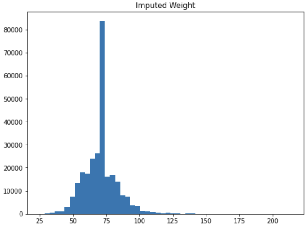
In this case we can start to see the risk of imputation. There are so many missing values that imputing the mean causes a spike in the middle of the data. If we were to feed this variable to a model it would think that the majority of Olympic athletes are around 70 inches tall. This could be true, but this could also be a majorly misleading variable for the model.
Hopefully, this example shows the importance of understanding the impact of your modeling choices and the effect they will have on the outcome. If you’re ever unsure we recommend talking to your teammates. Getting a different opinion on a process can be very helpful!
There are lots of great resources to learn more about imputation. We included a few examples below for your reference:
Feature Engineering
Feature engineering is the idea of creating new variables, or features, that can be added to a model to help with predictive power. New features are often very impactful but may be difficult to craft. This is an area where a subject matter expert’s (SME) knowledge can come in very handy.
When building new features, it’s important to have a way to compare them. Usually this involves building a baseline model and then seeing if a feature improves its accuracy. There is also a ton of articles written around the idea of feature selection. However, for this example we are going to walk through the ideation phase of feature engineering.
Going back to our Olympics data we can see that we have the columns below to work with:
import pandas as pd
import seaborn as sns
import matplotlib.pyplot as plt
import numpy as np

init_data = pd.read_csv('/depot/datamine/data/olympics/athlete_events.csv')

print(init_data.columns)
Index(['ID', 'Name', 'Sex', 'Age', 'Height', 'Weight', 'Team', 'NOC', 'Games',
'Year', 'Season', 'City', 'Sport', 'Event', 'Medal'],
dtype='object')
If our modeling goal is predicting the number of medals for specific countries, we would ideate on other factors that could help the model learn these trends. These could be built off data that we have in the dataset or imported from other datasets. A few potential feature examples are included below:
-
Importing external data on physical fitness tests in schools. Maybe the better the school age fitness the more Olympic success.
-
Creating a distance from the equator measurement. Maybe Olympics that are closer to the equator are hotter and support different outcomes.
-
Use the
Agevariable to create amean_age_by_teammeasurement. Maybe differences in average age drive differences in Olympic performance.
These are all random ideas. Your job as an analyst would be to come up with these hypotheses and then prove or disprove them with data. This also shows why a SME can be so helpful. Instead of me just guessing at these important factors imagine if you could talk to an Olympic athlete or coach. Their input could make a world of difference!